TL;DR
Below, you can find a quick summary of key points about density matrix:
- What is a density matrix?
A density matrix is a representation of a linear operator (or density operator) that describes the statistical state of a quantum system. It generalizes the wavefunction approach by representing pure coherent states and mixed classical ensembles of states.
- Is a density matrix Hermitian?
Yes, a density matrix is always Hermitian, satisfying the property . This property is physically required to ensure that all measurement expectation values are real numbers and that diagonal elements correspond to valid classical probabilities.
- How do you calculate a density matrix?
To calculate a density matrix, find the pure state vectors of the system and their classical probabilities . Compute the outer product for each state by multiplying the column vector by its conjugate transpose row vector, then sum the weighted outer products.
- What is the difference between a density matrix and a density operator?
A density operator and a density matrix refer to the same physical object. The density operator is the abstract linear operator acting on the Hilbert space, while the density matrix is its coordinate representation after choosing a specific orthonormal basis.
- What is the density matrix used for in quantum mechanics?
In quantum mechanics, the density matrix is used to calculate expectation values of observables and to model mixed states arising from noise or thermal variations. It is widely used in quantum computing to track decoherence, in statistical mechanics to represent thermal ensembles, and in the analysis of entangled subsystems.
- What is a reduced density matrix?
A reduced density matrix describes a subsystem’s quantum state within a larger, entangled system. It is calculated by tracing out other subsystems’ degrees of freedom, isolating the local state for analysis.
Table of Contents
In the classical world, particles possess definite positions and velocities. Quantum mechanics offers a richer picture. The density matrix mathematically describes pure and mixed quantum states, providing insights from quantum decoherence to quantum computing.
In this article, we will walk you through everything you need to know about the density matrix.
Here is what we will cover:
- What is a density matrix?
- Properties of a density matrix
- How to calculate a density matrix
- Reduced density matrix and reduced density operator
- Density matrix in quantum mechanics
- Density matrix vs wavefunction
What is a density matrix?
A density matrix is a representation of a linear operator, called the density operator, acting on the system’s Hilbert space (an abstract vector space) that describes its physical state.
Wavefunctions describe pure states where the quantum state is fully known. A density matrix can describe both pure states and mixed states, where there is some uncertainty about which quantum state the system is in.
John von Neumann introduced this idea in 1927 to bridge the gap between quantum mechanics and statistical physics.
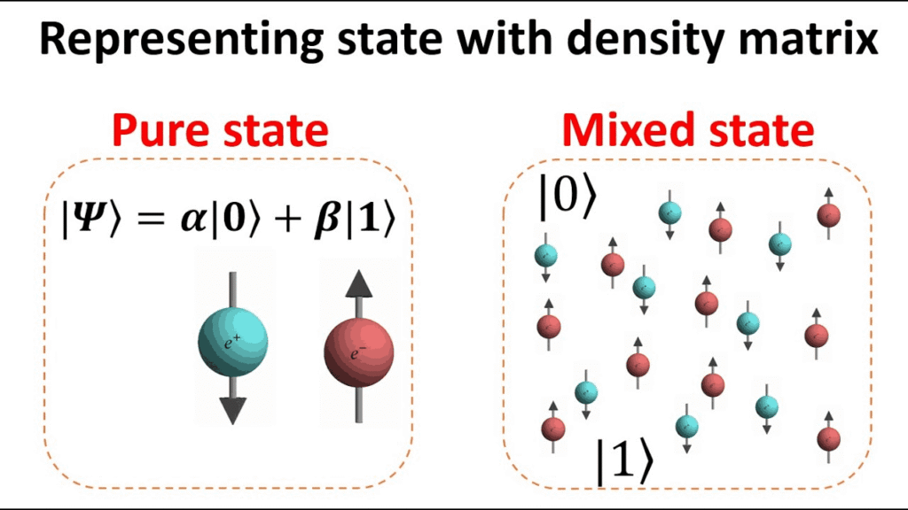
Here is a simple way to understand a mixed state. If you prepare a qubit using a machine. Half of the time, the machine prepares the qubit in state ∣0⟩. The other half, it prepares the qubit in state ∣1⟩.
You receive the qubit, but you do not know which state the machine prepared in a particular run. You only know the probabilities:
and
A single wavefunction cannot represent this classical uncertainty. A density matrix can describe the complete situation by combining the possible quantum states with their probabilities.
The density operator and density matrix refer to the same thing. A density operator is the general mathematical operation that describes the quantum state. When we choose a basis and write that operator as a table of numbers, we get the density matrix.
Density matrices are also useful for systems made of multiple quantum parts. For example, two qubits can become entangled. The complete two-qubit system may be in a pure state, while one qubit considered on its own appears to be in a mixed state.
Simply put, a density matrix lets us describe both the complete quantum system and its individual parts.
The general formula of a density matrix is:
Here:
- represents the density matrix.
- is the probability of the system being prepared in state .
- represents a possible quantum state.
- is the conjugate transpose of .
- creates a matrix that represents that pure state.
The formula says: take every possible quantum state, multiply it by the probability of that state occurring, and combine the results into one matrix.
Because represents probabilities, all probabilities must add up to 1:
Each probability must also be between 0 and 1:
For example, if a qubit has a 50% chance of being in and a 50% chance of being in , then:
and:
Properties of a density matrix
A density matrix must follow a few mathematical rules to represent a valid quantum state. These rules make sure that the matrix gives real and valid probabilities when we use it to predict measurement results.
The main properties of a density matrix are Hermiticity, a trace of 1, positive semi-definiteness, and a valid purity value.
Is a density matrix hermitian?
Yes. A density matrix is always Hermitian. This means the matrix is equal to its conjugate transpose: . The symbol means the conjugate transpose of the density matrix.
The trace must equal 1.
The trace of the density matrix must always be equal to one, ensuring that the probabilities of all possible states sum to unity:
A density matrix must be positive semi-definite.
For any state vector in the Hilbert space, the expectation value must be non-negative: , which is written as . This prevents any physical state from having a negative probability of occurrence.
Purity tells us whether a state is pure or mixed.
The trace of the squared density matrix is less than or equal to one: . The value equals 1 if and only if the state is pure, and is strictly less than 1 if the state is mixed ( means the trace (sum of the numbers on the matrix main diagonal)). For a system of dimension d, the maximally mixed state reaches the minimum value of .
For example, consider the pure state (we know exactly which state the qubit is in). Its density matrix is:
Squaring the matrix gives:
So:
So, ∣0⟩ is a pure state.
Now consider the 50/50 mixed state:
Squaring it gives:
The purity is: . Because the state is mixed.
For a quantum system with dimension d, the lowest possible purity is: . This value represents a maximally mixed state, where the system has the greatest possible uncertainty among its d basis states.
How to calculate a density matrix (worked examples)
To calculate a density matrix, take each possible quantum state, convert it into a matrix, multiply that matrix by the probability of the state occurring, and then add the matrices together.
Here are the steps you need to follow:
- Identify the possible quantum states. Write each state as a normalized state vector .
- Find the probability of each state. Assign a probability to every possible state. All probabilities must add up to 1.
- Create the outer product. Multiply each state vector by its conjugate transpose :
- Multiply each matrix by its probability. For each state, calculate:
- Add all the matrices together. The result is the final density matrix:
Now, let’s see how this calculation works with actual qubits.
Example 1: Pure state (qubit |0⟩)
Suppose we prepare a qubit in state .
Because we know exactly which state the qubit is in, it is a pure state. The probability of state is:
The state is written as a column vector:
Its conjugate transpose, called a bra vector, is:
Now multiply the column vector by the row vector:
The result is:
This is the density matrix for the pure state . What does the matrix tell us? Look at the diagonal values:
The value 1 means there is a 100% probability of finding the qubit in state . The value 0 means there is no probability of finding it in state .
So, the matrix density represents the known state of the qubit.
Example 2: Mixed state (50/50 statistical mixture)
Now imagine a machine prepares a qubit in one of two states:
- 50% of the time, it prepares .
- 50% of the time, it prepares .
The probabilities are:
and
You receive a qubit from the machine, but you do not know which state it prepared. This is a mixed state.
We already know the density matrix for :
Now calculate the matrix for .
The state vector is:
Its bra vector is:
The outer product is:
Because each state has a probability of 0.5, multiply both matrices by 0.5 and add them:
This gives:
We can also write it as:
where is the 2×2 identity matrix. This density matrix tells us that the qubit has a 50% chance of being in and a 50% chance of being in . Because neither state is more likely than the other, this is called a maximally mixed state.
Example 3: Bloch sphere representation
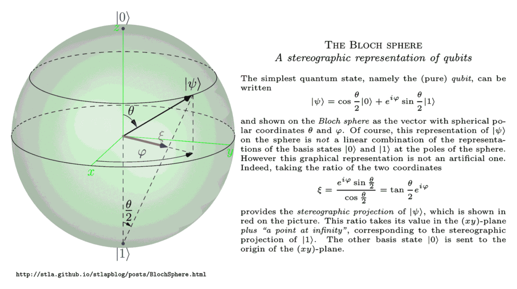
The Bloch sphere gives us a visual way to represent the state of a single qubit. Every valid 2×2 density matrix for a qubit can be represented by a point on or inside the Bloch sphere.
The density matrix formula is:
We can expand the formula as:
Here, is called the Bloch vector:
You can think of , , and as the coordinates of the quantum state on or inside the Bloch sphere.
The symbols represent the three Pauli matrices:
To find the Bloch vector coordinates from a density matrix, calculate:
For the pure state:
the calculations give:
So:
This places the |+⟩ state on the positive x-axis of the Bloch sphere. The location of a state also tells us something about its purity. Pure states sit on the surface of the Bloch sphere. Mixed states sit inside the sphere. The maximally mixed state sits exactly at the center.
Reduced density matrix and reduced density operator
A reduced density matrix describes one part of a larger quantum system. The term reduced density operator refers to the same mathematical object.
For example, imagine a quantum system with two qubits, A and B. The complete density matrix describes both qubits together. But what if you only want to study qubit A?
You can remove the information about qubit B using a mathematical operation called the partial trace (ignoring one qubit mathematically so you can focus only on the other qubit). The result is the reduced density matrix of qubit A.
The formula is:
Here:
- is the density matrix of the complete two-qubit system.
- means taking the partial trace over qubit B.
- is the reduced density matrix of qubit A.
Why does a reduced density matrix matter?
The reduced density matrix is especially useful for studying quantum entanglement.
When two qubits are entangled, you cannot fully describe one qubit with its own wavefunction. The state of one qubit depends on its connection with the other qubit.
A reduced density operator solves this problem. It lets you describe the local state of one qubit even when that qubit belongs to a larger entangled system.
Worked example: Two-qubit entangled system
Consider two qubits, A and B, in the Bell state:
This is an entangled quantum state.
The formula tells us that the two qubits are connected in the following way: if we measure the first qubit as 0, the second qubit is also 0. If we measure the first qubit as 1, the second qubit is also 1.
Before measurement, the complete system is described by the Bell state.
To create its density matrix, we take the outer product:
Expanding the formula gives:
Using the basis:
the density matrix is:
This matrix describes qubits A and B together.
But suppose we only want to study qubit A. We take the partial trace over qubit B:
More explicitly:
The calculation uses the following rules:
The first two expressions equal 1 because the states match. The last two equal 0 because the states are different.
After applying these rules, the reduced density matrix becomes:
In matrix form:
or:
his is a maximally mixed state.
The result tells us something interesting. The complete two-qubit system is in a pure Bell state, but qubit A, when studied alone, has a 50% probability associated with ∣0⟩ and a 50% probability associated with ∣1⟩.
We can check this using purity. For the complete system:
so, the complete system is pure. For qubit A:
Because the purity is less than 1, the reduced state of qubit A is mixed.
The key idea is simple: the complete entangled system can be perfectly known, while one part of that system looks mixed when studied alone.
Density matrix vs Wavefunction
A wavefunction describes a quantum system in a pure state, while a density matrix can describe both pure and mixed states. This makes the density matrix a more general tool, especially when dealing with statistical uncertainty, quantum noise, thermal states, or part of an entangled system.
Here is the comparison table:
| Comparison | Wavefunction | Density Matrix |
|---|---|---|
| Physical Scope | Describes pure quantum states. | Describes both pure and mixed quantum states. |
| Mathematical Object | A state vector in a Hilbert space. | A positive semi-definite, Hermitian operator with trace 1. |
| Statistical Mixtures | Cannot directly represent a classical mixture of quantum states. | Represents statistical mixtures using probabilities. |
| Global Phase | Two wavefunctions that differ only by a global phase represent the same physical state. | Global phase cancels when constructing the density matrix. |
| Subsystem Representation | Cannot fully describe one part of an entangled system with a wavefunction alone. | Describes a subsystem using a reduced density matrix. |
| Time Evolution | For a closed system, follows the Schrödinger equation. | For a closed system, follows the von Neumann equation; open-system dynamics require more general equations. |
| Expectation Value | Calculated using | |
| Thermal States | Cannot generally represent a thermal mixed state with a single wavefunction. | Represents thermal states using a thermal density matrix. |
Density matrix in quantum mechanics
Real quantum systems are rarely completely isolated. Noise, temperature, and environmental interactions can change a quantum state.
A wavefunction alone cannot always describe these situations. A density matrix can represent pure states, mixed states, and quantum systems affected by noise.
Key applications of the density matrix in quantum mechanics inlcudes:
Quantum Computing
Quantum computers use qubits to store and process quantum information. However, real qubits are sensitive to noise and hardware errors. These problems can cause a qubit to lose its quantum properties over time.
Density matrices help researchers model these noisy qubits and understand how errors affect a quantum circuit. Engineers can use this information to test quantum error correction methods and study the behavior of quantum gates.
Developers can also work with density matrices through quantum programming languages and software frameworks. These tools let you simulate quantum states, model noise, and study how quantum circuits behave before running them on real quantum hardware.
Statistical Mechanics
Density matrices also help physicists study quantum systems affected by temperature.
For example, if a quantum system is in contact with a warm environment. The system can exchange energy with its surroundings, so it may not stay in one pure quantum state. Instead, different energy states can occur with different probabilities.
A thermal density matrix describes this situation:
Here:
- represents the thermal density matrix.
- describes the energy of the quantum system.
- connects the calculation to temperature.
- is a normalization value that ensures the total probability adds up to 1.
Key takeaways
The density matrix provid a unified mathematical language to describe both coherent quantum phenomena and classical statistical mixtures. Its primary benefits include:
- Modeling noisy quantum systems: It helps describe quantum systems that interact with their environment and lose quantum coherence through decoherence.
- Describing parts of entangled systems: A reduced density matrix lets you study one part of a larger entangled quantum system.
- Predicting measurement results: It helps calculate the expected value of measurements for pure, mixed, and thermal quantum states.
- Removing global phase: The global phase cancels automatically when a density matrix is created, so it does not affect the description of the physical quantum state.
QbitNeural
AI and quantum research, decoded.
Paper summaries, model releases, and QML breakthroughs written for practitioners.

Asad Iqbal is a technical writer and researcher at the intersection of AI, machine learning, and quantum computing. With an MSc in Physics and over five years writing for AI and data companies, he brings something rare to science communication: the ability to read a research paper, understand what it actually means, and explain it clearly to practitioners. He founded QbitNeural to cover the AI and quantum research landscape with practitioner-level depth.